Introduction
This page demonstrates the core functionality of CounterfactualTraining.jl: training models that produce more plausible and actionable counterfactual explanations by holding them directly accountable during training.
Mutability Protection
When generating counterfactual explanations, some features may be immutable (e.g., age, race) while others are mutable (e.g., debt, income). Without protection, the contrastive divergence penalty can inadvertently make models more sensitive to immutable features, which is undesirable.
The key insight is that the contrastive divergence penalty gradient with respect to coefficient θ_{y⁺,d} is:
∂/∂θ_{y⁺,d} div(x⁺, x′, y; θ) = x′_d − x⁺_d
Since immutable features tend to differ between classes, the penalty would exacerbate the model’s existing sensitivity to those features. By protecting (zeroing gradients on) immutable features during counterfactual generation, the model learns to be relatively more sensitive to mutable features — producing counterfactuals that are actionable rather than relying on changes to features that cannot actually be changed.
Domain constraints are also applied to keep counterfactuals within plausible ranges for each feature.
Setup
using CounterfactualTraining
using CounterfactualTraining.Native
using CounterfactualExplanations
using Flux
using Plots
using Plots.PlotMeasures
using Random

Random.seed!(42)
gr()
Data
We use a linearly separable synthetic dataset of two Gaussian blobs (cluster standard deviation 0.5). Feature 1 — “Existing Debt” — and feature 2 — “Age” — can each be declared mutable (:both) or immutable (:none) depending on the experiment.
# Linearly separable synthetic data (two Gaussian blobs, std=0.5):
N = 3000
centers = Float32[0.0 0.0; 5.0 5.0]
n1 = N ÷ 2
n2 = N - n1
X1 = 0.5f0 .* randn(Float32, n1, 2) .+ centers[1:1, :]
X2 = 0.5f0 .* randn(Float32, n2, 2) .+ centers[2:2, :]
X = permutedims(vcat(X1, X2))              # 2 × N (features × observations)
y = vcat(fill(1, n1), fill(2, n2))

# Shuffle:
perm = randperm(N)
X, y = X[:, perm], y[perm]

y_onehot = Flux.onehotbatch(y, 1:2)
train_set = Flux.DataLoader((X, y_onehot); batchsize=50, shuffle=true)
Experiments
We train four models under different combinations of training objective and mutability constraints:
- (a)
VanillaObjective, both features mutable — standard training, no CF penalty. - (b)
FullObjective, both features mutable — CF training, no immutable feature to protect. - (c)
VanillaObjective, Age immutable — standard training; CFs may still move the immutable feature. - (d)
FullObjective, Age immutable — CF training with mutability protection.
All models share the same architecture: a multi-layer perceptron with one hidden layer of 32 ReLU units. We use AMSGrad and NativeGenerator for fast, batched counterfactual generation.
specs = [
    ("(a)", VanillaObjective(; needs_ce=false), [:both, :both]),
    ("(b)", FullObjective(lambda=Float32[1.0, 0.5, 0.01, 0.1]), [:both, :both]),
    ("(c)", VanillaObjective(; needs_ce=false), [:both, :none]),
    ("(d)", FullObjective(lambda=Float32[1.0, 0.5, 0.01, 0.1]), [:both, :none]),
]

generator = NativeGenerator()

models = []
ce_datasets = []

for (title, obj, mutability) in specs
    model = Chain(Dense(2, 32, relu), Dense(32, 2))
    opt_state = Flux.setup(Flux.Adam(), model)
    domain = CounterfactualTraining.infer_domain_constraints(X)
    data = CounterfactualData(X, y; domain=domain, mutability=mutability)

    model, log = counterfactual_training(
        obj, model, generator, train_set, opt_state;
        nepochs=100, maxiter=30, burnin=0.0f0,
        decision_threshold=0.75f0,
        mutability=mutability, domain=domain, verbose=0,
    )

    push!(models, model)
    push!(ce_datasets, data)
end
Counterfactual Generation
For each trained model we generate counterfactuals for 100 samples from class 1, targeting class 2 — matching the one-directional setup in the paper.
idx1 = findall(==(2), y)[1:100]
X_test = X[:, idx1]
targets = fill(1, length(idx1))

all_cfs = []
for i in eachindex(models)
    cfs, _, converged, _ = generate_counterfactuals!(
        models[i], X_test, targets, ce_datasets[i], generator;
        maxiter=100, decision_threshold=1.0f0,
    )
    push!(all_cfs, cfs)
end
Results
_xlab = "Existing Debt"
_ylab = "Age"

# Subsample background data for plotting:
idx_plot = randperm(size(X, 2))[1:min(500, size(X, 2))]
X_bg = X[:, idx_plot]
y_bg = y[idx_plot]

# Grid for decision boundary contour:
x1_range = range(minimum(X[1, :]), maximum(X[1, :]); length=50)
x2_range = range(minimum(X[2, :]), maximum(X[2, :]); length=50)

plts = []
for (i, (title, obj, mutability)) in enumerate(specs)
    cfs = all_cfs[i]
    yhat0 = vec(Flux.onecold(models[i](X_test)))
    yhat = vec(Flux.onecold(models[i](cfs)))
    idx_plotted = (yhat0 .== 1) .| (yhat0 .== 2)

    xlab = mutability[1] == :both ? "$_xlab (mutable)" : "$_xlab (immutable)"
    ylab = mutability[2] == :both ? "$_ylab (mutable)" : "$_ylab (immutable)"

    plt = scatter(
        X_bg[1, y_bg .== 1], X_bg[2, y_bg .== 1];
        color=1, ms=2, label=false,
        xlabel=xlab, ylabel=ylab,
        axis=nothing, legend=false, title=title,
    )
    scatter!(plt, X_bg[1, y_bg .== 2], X_bg[2, y_bg .== 2]; color=2, ms=2, label=false)

    # Linear decision boundary approximation (contour at p=0.5):
    Z = [Flux.softmax(models[i]([x1, x2]))[1] for x1 in x1_range, x2 in x2_range]
    contour!(plt, x1_range, x2_range, Z'; levels=[0.5], lw=5, color=:black, label=false)

    if any(idx_plotted)
        # Directional arrows from factual to counterfactual:
        u = cfs[1, idx_plotted] .- X_test[1, idx_plotted]
        v = cfs[2, idx_plotted] .- X_test[2, idx_plotted]
        quiver!(
            plt, X_test[1, idx_plotted], X_test[2, idx_plotted];
            quiver=(u, v), color=:gray, alpha=0.5, label=false,
        )

        # CF endpoints:
        scatter!(
            plt, cfs[1, idx_plotted], cfs[2, idx_plotted];
            ms=8, shape=:star, color=yhat[idx_plotted],
            group=yhat[idx_plotted], mscolor=yhat0[idx_plotted], label=false,
        )
    end
    push!(plts, plt)
end

plt = plot(
    plts...;
    layout=(1, 4),
    size=(1150, 250),
    left_margin=10mm, bottom_margin=5mm,
    top_margin=3mm, right_margin=10mm,
)
plt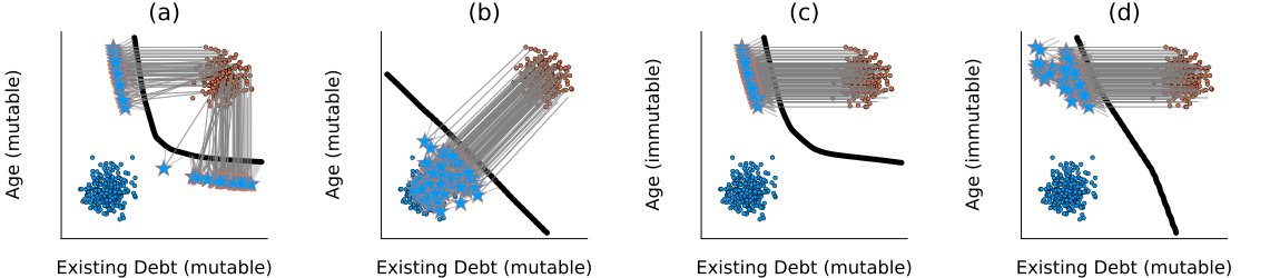
Only panel (d) — counterfactual training with mutability protection on the immutable feature — produces counterfactuals that move primarily along the mutable feature (Existing Debt), leaving the immutable feature (Age) relatively unchanged. The model has learned to be less sensitive to the immutable feature, producing counterfactuals that are more actionable.