Training on GPU
This page demonstrates GPU training with the Native submodule of CounterfactualTraining.jl.
Two Training Approaches
The package provides two training approaches that share the same counterfactual_training entry point (dispatch is based on the generator type):
Research branch (non-native): Uses
CounterfactualExplanations.jlstructs (GenericGenerator,CounterfactualExplanation) andTaijaParallel.parallelizefor per-sample counterfactual generation. Heavier and slower, but fully featured. Dispatched whengeneratoris not aNativeGenerator.Performance branch (
Nativesubmodule): A lightweight, batched, GPU-friendly generator (NativeGenerator) that operates directly onD×Nmatrices without allocatingCounterfactualExplanationobjects per sample. Much faster and GPU-compatible. Dispatched whengenerator isa NativeGenerator.
The Native branch was added as part of the performance optimization effort and is the recommended approach for most use cases.
Setup
using CounterfactualTraining
using CounterfactualTraining.Native
using CounterfactualExplanations
using Flux
using Metalhead
using Plots
using Random
using MLDatasets
using JLD2
using Statistics

Random.seed!(42)
gr()
GPU Detection
The code below detects available GPU backends (CUDA or AMDGPU) and falls back to CPU if none is available. This makes the example runnable in any environment, including CI.
has_gpu = false
device = identity

# Try CUDA
try
    using CUDA
    if CUDA.functional()
        global has_gpu = true
        global device = Flux.gpu
    end
catch
end

# Try AMD
if !has_gpu
    try
        using AMDGPU
        if AMDGPU.functional()
            global has_gpu = true
            global device = Flux.gpu
        end
    catch
    end
end

if has_gpu
    @info "GPU detected — training will run on GPU."
else
    @info "No GPU available — training will run on CPU."
end
GPU Memory Management
Running two heavy trainings back-to-back in one process can silently starve the GPU. On AMDGPUs the freed ROCArrays are cached in a HIP memory pool that is only released to the driver under memory pressure, so the FullObjective counterfactual search can leave the pool seemingly full even after the arrays are freed. Under memory stress a subsequent allocation can stall on a device synchronization and hang the whole pipeline with no error — GPU utilisation drops to ~0% and only repeated ^C recovers it.
AMDGPU.eager_gc!(true) proactively collects before large allocations (at ~75% pool pressure), which prevents these out-of-memory stalls in allocation-heavy workloads:
if isdefined(Main, :AMDGPU)
    AMDGPU.eager_gc!(true)
    @info "AMDGPU ready — GPU memory (used): $(round(AMDGPU.used() / 2^30; digits=2)) GiB"
else
    @info "No AMDGPU backend in use — GPU memory management skipped."
end
Loading MNIST
We load MNIST via MLDatasets.jl, flatten the 28×28 images to 784-dimensional vectors, and normalize pixel values to [-1, 1]. A subset of 5,000 samples is used to keep the example fast.
train_data = MLDatasets.MNIST(; split=:train)
X = Float32.(reshape(train_data.features, 784, :)) .* 2f0 .- 1f0
y = train_data.targets .+ 1  # convert 0-9 labels to 1-10

idx = shuffle(1:size(X, 2))[1:5000]
X, y = X[:, idx], y[idx]

domain = [(-1.0f0, 1.0f0) for _ in 1:784]
y_onehot = Flux.onehotbatch(y, 1:10)

# Keep the data on the device so the training loop's `input |> device` is a
# cheap no-op instead of a per-batch H2D copy.
X = X |> device
y_onehot = y_onehot |> device
train_set = Flux.DataLoader((X, y_onehot); batchsize=128, shuffle=true)
Model
We use a ResNet-18 from Metalhead.jl, configured for single-channel 28×28 MNIST inputs and 10 output classes. The native counterfactual pipeline operates on flattened D×N matrices throughout (see generate_counterfactuals! in src/native/training.jl), so we wrap the backbone in a Chain that reshapes the 784-dimensional input back to 28×28×1×N before the first convolution. This keeps the counterfactual search in pixel space, where the per-pixel domain bounds ((-1, 1)) and mutability constraints remain valid, without requiring changes to the matrix-typed pipeline.
backbone = ResNet(18; inchannels=1, nclasses=10)
model = Chain(x -> reshape(x, 28, 28, 1, :), backbone)
Training
We compare two objectives to illustrate the overhead of the counterfactual pipeline: FullObjective (generates counterfactuals each epoch after burn-in) and VanillaObjective(; needs_ce=false) (standard training, no CF generation). Both runs use the same model, optimizer, and hyperparameters, and start from identical initial weights (Random.seed!(42) is re-seeded before constructing each model). The training log records time_taken per epoch in both branches, so we plot the per-epoch wall-clock time for the two objectives.
GPU memory-pressure
If you interested reproducing the computations in this tutorial, be mindful of hardware requirements (see Section 9).
To avoid the silent GPU memory-pressure hangs discussed above, the two expensive trainings are run in separate Julia processes, each saving its
logto disk; a third process loads both logs and produces the comparison figure. This mirrors how you would run them on your own machine and keeps each process on a fresh, un-fragmented GPU heap.Select the stage with the
CT_MODEenvironment variable:
CT_MODE=full— run theFullObjectivetraining, savedocs/src/data/gpu_full.jld2.CT_MODE=vanilla— run theVanillaObjectivetraining, savedocs/src/data/gpu_vanilla.jld2.CT_MODE=plot(default) — load both saved logs and build the figure (requires the two runs to have completed first).
CT_MODE = "plot"

nepochs = 25
verbose = 2
opt = Flux.Adam(1e-3)
nce = 1024
# cf_batchsize is a GPU-memory knob for the CF search; 128 (= nce, so no
# chunking) is fastest here — lower it only on memory-constrained GPUs.
cf_batchsize = 128
accuracy_every = div(nepochs, 10)
burnin = 0.2f0
burnin_epochs = Int(round(burnin * nepochs))
gen = NativeGenerator()
Full objective
if CT_MODE == "full"
    Random.seed!(42)
    model_full = Chain(x -> reshape(x, 28, 28, 1, :), ResNet(18; inchannels=1, nclasses=10))

    obj = FullObjective()
    opt_state = Flux.setup(opt, model_full);

    _, log_full = counterfactual_training(
        obj, model_full, gen, train_set, opt_state;
        device, nepochs, domain, verbose, accuracy_every,
        nce, cf_batchsize,
        maxiter=30, burnin=burnin
    )
    jldsave("docs/src/data/gpu_full.jld2"; log=log_full)
    @info "Saved FullObjective log to docs/src/data/gpu_full.jld2"
    log_full = nothing  # release the log (and allow GPU arrays from the run to be collected)
    model_full = nothing
else
    @info "Skipping FullObjective training (CT_MODE = $CT_MODE)."
end
Vanilla objective
if CT_MODE == "vanilla"
    Random.seed!(42)
    model_vanilla = Chain(x -> reshape(x, 28, 28, 1, :), ResNet(18; inchannels=1, nclasses=10))

    obj_vanilla = VanillaObjective(; needs_ce=false)
    opt_state_vanilla = Flux.setup(opt, model_vanilla);

    _, log_vanilla = counterfactual_training(
        obj_vanilla, model_vanilla, gen, train_set, opt_state_vanilla;
        device, nepochs, domain, verbose, accuracy_every,
    )
    jldsave("docs/src/data/gpu_vanilla.jld2"; log=log_vanilla)
    @info "Saved VanillaObjective log to docs/src/data/gpu_vanilla.jld2"
    log_vanilla = nothing
    model_vanilla = nothing
else
    @info "Skipping VanillaObjective training (CT_MODE = $CT_MODE)."
end
Timing and accuracy comparison
full_path = "docs/src/data/gpu_full.jld2"
vanilla_path = "docs/src/data/gpu_vanilla.jld2"

if isfile(full_path) && isfile(vanilla_path)
    log_full = JLD2.load(full_path, "log")
    log_vanilla = JLD2.load(vanilla_path, "log")

    # Timing
    t_full = [l.time_taken for l in log_full]
    t_vanilla = [l.time_taken for l in log_vanilla]

    # Post-burn-in per-epoch averages (horizontal guide lines)
    post = (burnin_epochs + 1):length(t_full)
    mean_full = mean(t_full[post])
    mean_vanilla = mean(t_vanilla[post])

    # Accuracy (non-nothing epochs only — depends on accuracy_every)
    epochs_acc = [i for (i, l) in enumerate(log_full) if !isnothing(l.acc)]
    acc_full = [l.acc for l in log_full if !isnothing(l.acc)]
    acc_vanilla = [l.acc for l in log_vanilla if !isnothing(l.acc)]

    # Implausibility trajectory (Full objective only; recorded after burn-in)
    epochs_impl = [i for (i, l) in enumerate(log_full) if !isnothing(l.implaus)]
    impl_full = [l.implaus for l in log_full if !isnothing(l.implaus)]

    # Series colors (shared between curve, average line and annotation)
    c_full = :steelblue
    c_vanilla = :darkorange

    plt1 = plot(
        1:length(t_full), t_full;
        label="Full objective",
        xlabel="Epoch", ylabel="Time per epoch (s)",
        lw=2, color=c_full,
    )
    plot!(plt1, 1:length(t_vanilla), t_vanilla; label="Vanilla objective", lw=2, color=c_vanilla)
    vline!(plt1, [burnin_epochs]; label="Burn-in ends", ls=:dash, color=:black)
    hline!(plt1, [mean_full]; label="Full post-burn-in avg", ls=:dot, lw=2, color=c_full)
    hline!(plt1, [mean_vanilla]; label="Vanilla post-burn-in avg", ls=:dot, lw=2, color=c_vanilla)
    annotate!(
        (length(t_full) / 2, mean_full,
            text(string("Full avg: ", round(mean_full; digits=1)), :center, 8, c_full)),
        (length(t_vanilla) / 2, mean_vanilla,
            text(string("Vanilla avg: ", round(mean_vanilla; digits=1)), :center, 8, c_vanilla)),
    )

    plt2 = plot(
        epochs_acc, acc_full;
        label="Full objective",
        xlabel="Epoch", ylabel="Training accuracy", lw=2,
    )
    plot!(plt2, epochs_acc, acc_vanilla; label="Vanilla objective", lw=2)
    vline!(plt2, [burnin_epochs]; label="Burn-in ends", ls=:dash, color=:black)

    plt3 = plot(
        epochs_impl, impl_full;
        label="Implausibility",
        xlabel="Epoch", ylabel="Implausibility (energy diff.)", lw=2,
        color=:green,
    )
    vline!(plt3, [burnin_epochs]; label="Burn-in ends", ls=:dash, color=:black)

    combined = plot(
        plt1, plt2, plt3;
        layout=(1, 3),
        size=(1350, 400),
        bottom_margin=10Plots.mm,
        left_margin=10Plots.mm,
    )
    savefig(combined, "docs/src/assets/gpu.svg")
    @info "Saved comparison plot to docs/src/assets/gpu.svg"
else
    @warn "Missing saved logs. Run CT_MODE=full and CT_MODE=vanilla first (each in its own process). Found: full=$(isfile(full_path)), vanilla=$(isfile(vanilla_path))"
end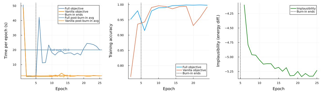
Per-epoch wall-clock time, training accuracy, and implausibility trajectory for the full and vanilla objectives.
The figure above compares the two objectives across three panels. The left panel shows per-epoch wall-clock time, with dashed lines marking the end of burn-in and dotted horizontal lines (with annotated values) giving each objective’s post-burn-in per-epoch average. The middle panel shows training accuracy, and the right panel shows the trajectory of the implausibility (energy differential) loss for the full objective. The gap between the two curves in the left panel reflects the cost of generating counterfactuals each epoch (the per-sample batched search in generate_native!). Expect the difference to appear only after the burn-in fraction, since VanillaObjective(; needs_ce=false) short-circuits CF generation entirely via needs_counterfactuals. The middle panel confirms that both objectives achieve comparable training accuracy, indicating that the counterfactual regularization does not degrade the discriminative performance of the model, while the implausibility trajectory shows the full objective steadily lowering the energy differential as training proceeds.
Performance tips
- Keep the full dataset on the device before building the
DataLoader(as shown above) so the training loop’sinput |> deviceis a no-op rather than a per-batch copy. - Set
cf_batchsizeas large as memory allows to avoid chunking the counterfactual search (e.g.128whennce = 128). Lower it only on memory-constrained GPUs. - Use
accuracy_every(e.g.div(nepochs, 5)) to skip per-epoch accuracy when wall-clock time matters. - For BatchNorm models, consider
fuse_cf_forwards = trueonly if slightly different batch statistics are acceptable (it fuses the three counterfactual forward passes into one). - Run the two trainings in separate processes to avoid GPU memory-pressure hangs. This page does so via
CT_MODE— runCT_MODE=full quarto render docs/src/gpu.qmd, then (in a fresh process)CT_MODE=vanilla quarto render docs/src/gpu.qmd, thenquarto render docs/src/gpu.qmd(defaultCT_MODE=plot) to build the figure. This is equivalent to launching the two runs as independent Julia sessions. - On AMDGPUs, enable
AMDGPU.eager_gc!(true)in each process to collect before large allocations at ~75% pool pressure (see GPU Memory Management). Because each run now gets a fresh process, in-processAMDGPU.HIP.reclaim()between runs is no longer necessary, though it is still useful if you keep several heavy workloads in one session.
Hardware
These experiments were run on a Framework Desktop with 64GB unified RAM (AMD Ryzen AI Max+ 395).